

categorical input – categorical output
260320201223
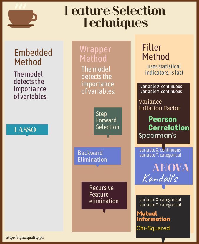
In this case, statistical methods are used:
We always have continuous and discrete variables in the data set.
This procedure applies to the relations of discrete independent variables in relation to discrete result variables.
Below I show the analysis of discrete variables when the resulting value is discrete.

data from the Titanic disaster
import pandas as pd

df = pd.read_csv('/home/wojciech/Pulpit/1/kaggletrain.csv',sep=',',nrows=1000000)

print()
print(df.shape)
print()
print(df.columns)
We choose only discrete variables
Because we are testing discrete data with discrete data, there must be only discrete variables of type ‘object’ in the test set.
The following code throws out all independent variables identified by Pandas as continuous. This must be verified and possibly converted to a discrete format.
The ‘object’ format is the most economical of formats in terms of memory usage.
import numpy as np

continuous_vars = df.describe().columns
df[continuous_vars].agg(['nunique','dtypes','min','max','median'])
We are replacing detected discrete variables with the ‘object’ format
df['Survived'] = df['Survived'].astype(object)
df['Pclass'] = df['Pclass'].astype(object)
df['SibSp'] = df['SibSp'].astype(object)
df['Parch'] = df['Parch'].astype(object)
I can make a discrete variable out of the Age variable
Ewa = ['dziecko', 'młody','średni','starszy','stary']

df['Age2'] = pd.qcut(df['Age'],5, labels=Ewa)
df['Age2'] = df['Age2'].astype('object')
df[['Age','Age2']].sample(3)
Once again we check what could have been wrong.
import numpy as np
continuous_vars = df.describe().columns
df[continuous_vars].agg(['nunique','dtypes','min','max','median'])
Checking categorical variables
categorical_vars = df.describe(include=["object"]).columns

import numpy as np

df[categorical_vars].agg(['nunique','dtypes','min','max','median'])
Checking and clearing empty records in discrete variables
df[categorical_vars].isnull().sum()
Deleting unnecessary columns
del df['Cabin']
del df['Name']
del df['Ticket']
categorical_vars = df.describe(include=["object"]).columns
df[categorical_vars].isnull().sum()
print(df.shape)
df=df.dropna(how='any')
print(df.shape)
df[categorical_vars].isnull().sum()
#del df['id']
categorical_vars
categorical_vars = ['Pclass','Sex','SibSp','Parch','Embarked','Age2','Survived']
print(df.info(memory_usage='deep'))
df[categorical_vars].head(3)
Coding of discrete variables
from sklearn.preprocessing import OrdinalEncoder
from sklearn.preprocessing import LabelEncoder

df2 = df[categorical_vars].apply(LabelEncoder().fit_transform)
df2.head(4)
I’m creating an array with dataframe
## tworzę array z dataframe
dataset = df2.values
dataset[:3]
Divides data into describing variables and a result variable
X = dataset[:, :-1]
y = dataset[:,-1]
y[:25]
We divide the data into a training and test set
from sklearn.model_selection import train_test_split

X_train, X_test, y_train, y_test = train_test_split(X, y, test_size=0.33, random_state=1)

print('Train', X_train.shape, y_train.shape)
print('Test', X_test.shape, y_test.shape)
X_train[:5]
y_train[:35]
Definition
# Classification Assessment
def Classification_Assessment(model ,Xtrain, ytrain, Xtest, ytest, y_pred):
    import matplotlib.pyplot as plt
    from sklearn import metrics
    from sklearn.metrics import classification_report, confusion_matrix
    from sklearn.metrics import confusion_matrix, log_loss, auc, roc_curve, roc_auc_score, recall_score, precision_recall_curve
    from sklearn.metrics import make_scorer, precision_score, fbeta_score, f1_score, classification_report

    print("Recall Training data:     ", np.round(recall_score(ytrain, model.predict(Xtrain)), decimals=4))
    print("Precision Training data:  ", np.round(precision_score(ytrain, model.predict(Xtrain)), decimals=4))
    print("----------------------------------------------------------------------")
    print("Recall Test data:         ", np.round(recall_score(ytest, model.predict(Xtest)), decimals=4))
    print("Precision Test data:      ", np.round(precision_score(ytest, model.predict(Xtest)), decimals=4))
    print("----------------------------------------------------------------------")
    print("Confusion Matrix Test data")
    print(confusion_matrix(ytest, model.predict(Xtest)))
    print("----------------------------------------------------------------------")
    print(classification_report(ytest, model.predict(Xtest)))

    y_pred_proba = model.predict_proba(Xtest)[::,1]
    fpr, tpr, _ = metrics.roc_curve(ytest,  y_pred)
    auc = metrics.roc_auc_score(ytest, y_pred)
    plt.plot(fpr, tpr, label='Logistic Regression (auc = plt.xlabel('False Positive Rate',color='grey', fontsize = 13)
    plt.ylabel('True Positive Rate',color='grey', fontsize = 13)
    plt.title('Receiver operating characteristic')
    plt.legend(loc="lower right")
    plt.legend(loc=4)
    plt.plot([0, 1], [0, 1],'r--')
    plt.show()
    print('auc',auc)
Model Logistic Regression on ordinary data
import numpy as np
from sklearn import model_selection
from sklearn.pipeline import make_pipeline
from sklearn.linear_model import LogisticRegression
from sklearn.model_selection import GridSearchCV

Parameteres = {'C': np.power(10.0, np.arange(-3, 3))}
LR = LogisticRegression(warm_start = True)
LR_Grid = GridSearchCV(LR, param_grid = Parameteres, scoring = 'roc_auc', n_jobs = -1, cv=2)

LR_Grid.fit(X_train, y_train)
y_pred_LRC = LR_Grid.predict(X_test)
Classification_Assessment(LR_Grid ,X_train, y_train, X_test, y_test, y_pred_LRC)

Mutual Information Feature Selection: Mutual_info_classif ()
Mmutual Information is usually used in the construction of decision trees for selecting variables.
from sklearn.feature_selection import mutual_info_classif
from sklearn.feature_selection import SelectKBest


def select_features_MIC(X_train, y_train, X_test):
    MIC = SelectKBest(score_func=mutual_info_classif, k='all')
    MIC.fit(X_train, y_train)
    X_train_MIC = MIC.transform(X_train)
    X_test_MIC = MIC.transform(X_test)
    return X_train_MIC, X_test_MIC, MIC
import time
start_time = time.time() ## pomiar czasu: start pomiaru czasu
print(time.ctime())

X_train_MIC, X_test_MIC, MIC = select_features_MIC(X_train, y_train, X_test)

print('Time to complete the task')
print('minutes: ',
(time.time() - start_time)/60) ## koniec pomiaru czasu
Printing the results of the Mutual_info_classif () selection (the highest value is the best value)
df2.columns
for i in range(len(MIC.scores_)):
    print('Feature
importance_mic = np.round(MIC.scores_, decimals=3)
importance_mic
KOT_MIC = dict(zip(df2, importance_mic))
KOT_sorted_keys_MIC = sorted(KOT_MIC, key=KOT_MIC.get, reverse=True)

for r in KOT_sorted_keys_MIC:
    print (r, KOT_MIC[r])
KOT_MIC
import matplotlib.pyplot as plt

plt.bar(*zip(*KOT_MIC.items()))
plt.xticks(rotation=90)
plt.show

import seaborn as sns

sns.barplot(list(KOT_MIC.keys()), list(KOT_MIC.values()))
plt.title('Mutual Information Feature Selection')
plt.ylabel('variance')
plt.xlabel('independent variables')
plt.xticks(rotation=90)

Logistic regression for Mutual Information
Logistic regression is a good model for testing feature selection methods because it can work better if irrelevant features are removed from the model.
def red(text):
    print('33[31m', text, '33[0m', sep='')

from sklearn import metrics
from sklearn.linear_model import LogisticRegression
from sklearn.metrics import accuracy_score
from sklearn.metrics import classification_report, confusion_matrix
from sklearn.metrics import confusion_matrix, log_loss, auc, roc_curve, roc_auc_score, recall_score, precision_recall_curve
from sklearn.metrics import make_scorer, precision_score, fbeta_score, f1_score, classification_report

MIC_model = LogisticRegression(solver='lbfgs')
MIC_model.fit(X_train_MIC, y_train)
# evaluate the model
yMIC = MIC_model.predict(X_test_MIC)
Classification_Assessment(MIC_model ,X_train_MIC, y_train, X_test_MIC, y_test, yMIC)

Feature Selection by Chi-Squared
from sklearn.feature_selection import SelectKBest
from sklearn.feature_selection import chi2

def select_features_CH2(X_train, y_train, X_test):
    CH2 = SelectKBest(score_func=chi2, k=4)
    CH2.fit(X_train, y_train)
    X_train_CH2 = CH2.transform(X_train)
    X_test_CH2 = CH2.transform(X_test)
    return X_train_CH2, X_test_CH2, CH2
import time
start_time = time.time() ## pomiar czasu: start pomiaru czasu
print(time.ctime())

X_train_CH2, X_test_CH2, CH2 = select_features_CH2(X_train, y_train, X_test)

print('Time to complete the task')
print('minutes: ',
(time.time() - start_time)/60) ## koniec pomiaru czasu
Printing the results of the Chi-Squared selection (the highest value is the best value)
df2.columns
for i in range(len(CH2.scores_)):
    print('Feature
importance_CH2 = np.round(CH2.scores_, decimals=3)
importance_CH2

KOT_CH2 = dict(zip(df2, importance_CH2))
KOT_CH2_sorted_keys = sorted(KOT_CH2, key=KOT_CH2.get, reverse=True)

for r in KOT_CH2_sorted_keys:
    print (r, KOT_CH2[r])
import seaborn as sns

sns.barplot(list(KOT_CH2.keys()), list(KOT_CH2.values()))

plt.title('Chi-Squared Feature Selection')
plt.ylabel('variance')
plt.xlabel('independent variables')

plt.xticks(rotation=90)

Logistic regression for Chi-Squared
from sklearn import metrics
from sklearn.linear_model import LogisticRegression
from sklearn.metrics import accuracy_score
from sklearn.metrics import classification_report, confusion_matrix
from sklearn.metrics import confusion_matrix, log_loss, auc, roc_curve, roc_auc_score, recall_score, precision_recall_curve
from sklearn.metrics import make_scorer, precision_score, fbeta_score, f1_score, classification_report

CH2_model = LogisticRegression(solver='lbfgs')
CH2_model.fit(X_train_CH2, y_train)
# evaluate the model
yCH2 = CH2_model.predict(X_test_CH2)
Classification_Assessment(CH2_model ,X_train_CH2, y_train, X_test_CH2, y_test, yCH2)
