
May 2021 | Przegląd Zbożowo-Młynarski (Grain and Milling Review)
DATA SCIENCE IN THE MILLING INDUSTRY
A classification model is a model whose result is a discrete value (discrete variable), that is, one which does not have a continuous form (continuous variable). Continuous values, in turn, are values which can be expressed in the form of floating-point numbers. Discrete values are zero-one values, or values taking a larger but limited number of forms expressed by whole numbers, names, symbols or letters.
Most classification models do not tolerate variables in the form of a series of symbols or letters, and that is why, during the preparation of the data, they are compiled into the form of whole numbers.
In the new field which is data science, most models are categorical classification models. These are models answering questions such as: will a critical level be exceeded or not, will it rain or not, will the patient die or survive.
W-MOSZCZYNSKI pzm 5-21Supervised learning
The overwhelming number of data science models is carried out in the regime of supervised learning. In order to create an econometric model there must exist a series of independent variables and at least one dependent variable, also called the outcome variable. The independent variables, also called describing variables, may have a continuous form, such as temperature, humidity or weight, or a discrete form, such as the day of the week, sex, the full hour or the time of day.
What does supervised learning consist in?
Let us imagine that we already have the data, a dozen or so describing variables and a selected outcome variable. Supervised learning consists in dividing the original data set into a training set and a test set. It has become accepted that the training set constitutes about 70–80% of the size of the original set, while the rest, that is 20–30% of that set, constitutes the test set.
Ideally, the original data set is divided into a test set and a training set while preserving a similar statistical characteristic of the individual describing variables (e.g. the structure of the probability distribution). Both sets should therefore be statistically similar to each other.
Supervised learning consists in training the model on the training set, and then checking the effectiveness of the learning by substituting into the trained model the independent variables of the test set. Then the theoretical values obtained from the model are compared with the outcome values of the test set.
The cause-and-effect relationship of describing and outcome variables
The result of a classification model has a discrete form. For the model to be effective there must exist a significant informational connection between the describing variables and the outcome variable. Unfortunately, in the case of discrete variables there can be no question of measuring the cause-and-effect connection by means of ordinary Pearson correlation (Pearson’s correlation coefficient). When the independent and dependent variables have a discrete form (also called a categorical form), the cause-and-effect connection between them is measured by means of the Mutual Information or Chi-Squared method. When the describing variables have a continuous form, their influence on a discrete outcome variable is measured by the ANOVA algorithm or by Kendall’s method of interdependence (Kendall’s rank coefficient).
Assessing the quality of classification
Let us assume that we have managed to build a model which is able to indicate whether the grain at the purchasing point is infected with mould or not. At this stage of purchasing, the mould is not yet visible.
The model was trained on the training set on the basis of a dozen or so available variables such as colour, unit mass or humidity. Thanks to them the model is able to indicate which grain will soon become visibly mouldy.
Having a test set, we can assess what the accuracy of the model’s classification is. It is enough to substitute into the trained model the independent variables from the test set and in this way obtain theoretical results. By comparing the theoretical results with the laboratory results contained in the test set, we can quickly catch all the model’s classification errors.
In dichotomous classification models there are four possible assessments:
- True positive: the model correctly indicated mouldy grain as mouldy grain.
- True negative: the model correctly indicated healthy grain as healthy grain.
- False positive: the model indicated healthy grain as mouldy grain.
- False negative: the model indicated mouldy grain as healthy grain.
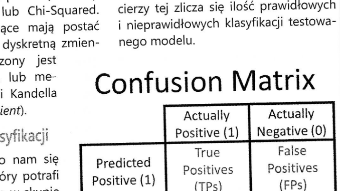
The compilation of the four classification states is called a confusion matrix, also known as an error matrix. In this matrix the number of correct and incorrect classifications of the tested model is counted.
It is difficult to assess the quality of classification by looking at the confusion matrix alone. That is why a series of assessment indicators has been devised, among which the two most important are: recall and precision.
Recall is an indicator based on the ratio of the quantity of correctly detected mouldy grain (classifications of the type: true positive) to the whole volume of mouldy grain which passed through the model (the sum of classifications of the type: true positive and false negative). It is simply the percentage share of detected mouldy grain in the total quantity of mouldy grain which was subjected to examination by the model. When recall amounts to 73%, this means that 27% of the mouldy grain was classified as healthy grain.
Precision works differently. It is the ratio of correctly classified mouldy grain (classifications of the type: true positive) to the whole sum of grain which the model indicated as mouldy grain. Precision therefore indicates what the share of really mouldy grain is in the grain which was classified by the model as mouldy. So, for example, a precision value of 82% means that 18% of healthy grain was regarded by the model as mouldy grain.
The problem of an unbalanced set of results
A classification model will work best when the volume of mouldy grain is comparable to the volume of healthy grain. Fortunately, mouldy grain is a rarity at the purchasing point. Let us assume that grain with invisible mould constitutes barely 1% of all the grain received at the purchasing point. There is therefore an enormous disproportion of healthy grain in relation to infected grain. In such a situation the model will not be able to make a correct classification. When we run the model it will easily indicate that all the grain received is healthy. Unfortunately, such is the logic of mathematical algorithms. They simplify reality, taking decisions on the basis of the calculus of probability. A model which decides that all the grain is healthy will have a very good relative assessment of the quality of classification, because the recall and precision indicators will show very low effectiveness equal to zero, and this algorithm will be useless to us.
Balancing the set of results
Classification models usually serve to track down rare phenomena, such as financial fraud, genetic defects, rare diseases or system errors.
The aim of classification is often to search for anomalies whose occurrence is extremely unique. For a classification model to be able to work correctly it must have a similar quantity of typical and unique phenomena. If there are as many typical phenomena as unique ones, the latter will no longer be unique. So we have a condition which seems impossible to fulfil. However, this curious condition can be fulfilled by applying one of two techniques: oversampling and undersampling.
The oversampling technique consists in creating in the training data set a great quantity of artificial unique events by copying them from real events registered in the training set. The quantity of typical variables should be similar. Thanks to this the model will not lose the importance of any of the categories.
The undersampling technique consists in eliminating from the training data set populations of typical events so that their number is close to the number of unique events. In econometrics the central limit theorem reigns, which indicates the widespread occurrence in nature of…
The use of classification models
Because of the radical character of their results, classification models are to some degree more effective than regression models, whose results have a continuous form. A typical application of regression models is forecasts of prices, temperature, pressure and other continuous magnitudes.
Regression models may, for example, indicate a forecast of prices on the exchange, whereas categorical classification models can only say whether the price will rise or fall. Classification models can also determine several classes of falls and rises, as a result of which the information will be more precise. It seems that the development of predictive techniques will rest more often on the forecast intervals offered by classification models than on the continuous values offered by regression models.
In the past, an enormous part of statistical analyses showed results in the form of probability intervals. This method was abandoned, because such results were difficult to interpret for ordinary people.
Wojciech Moszczyński
In collaboration with Ewa Moszczyńska
Wojciech Moszczyński — graduate of the Department of Econometrics and Statistics of Nicolaus Copernicus University in Toruń; specialist in econometrics, finance, data science, and management accounting. He specializes in the optimization of production and logistics processes. He conducts research in the area of the development and application of artificial intelligence. For years he has been engaged in the popularization of machine learning and data science in business environments.
Dodaj komentarz