
January 2023 | Przegląd Piekarski i Cukierniczy (Baking and Confectionery Review)
The time of superstitions and beliefs has passed irrevocably — or has it really?
More than once I have met excellent engineers who believed that „during a full moon” gas consumption is always higher, or that painting a machine red brings bad luck. Every such observation is valuable if one first verifies it by means of a statistical test before believing in it.
Checking with the „moss and fern” test is very simple. It is enough to make use of a free online calculator. If we check something statistically, we can talk about it further — this time seriously — and nobody will take us for storytellers talking about „full moons” and „mysterious powers”. Not to mention the fact that invoking the results of statistical tests may meet with recognition from analysts or accountants.
Prediction
One of the most important skills in running a bakery is inference and prediction. On the basis of our own experience we know, for example, that bread sells best on Mondays, Wednesdays and Saturdays. Thanks to this knowledge we plan a level of production which will cause the minimal level of returns. Unfortunately we do not always manage to hit the target with production. Every excessive level of production means thousands of złoty thrown away. Well, not exactly thrown away, but into breadcrumbs, raw material for thickening dough, or poultry feed. If we produce too little bread, we risk upsetting the local community. Every baker who has had such an episode knows what it means to upset half the town.
W-MOSZCZYNSKI ppic 1-23So it is worth applying oneself to predicting the future. We know, for example, that bread sells better on certain days of the week. To find out better how much should be produced, one can draw the average sales volume from all Mondays. The resulting number will be as good as the standard deviation accompanying it is good. If we find out that on average we sell 1000 loaves of bread on Mondays with a deviation of plus or minus 250 loaves, what should we do with this information? Should we produce 1250 loaves, and if sales dip we will be left with returns at the level of 500 loaves? That is, the returns will be at the level of half the average sale from all the Mondays of this year.
Not only the day of the week
From the above example it follows that other factors also influence bread sales. After reflection we conclude that the weather also has an influence. Specifically, the level of the perceived temperature, air humidity, and the level of precipitation. A series of further factors appear. For example, an approaching long weekend or the beginning of the holiday season. Changes in demand between the period before the tenth day of each month and after the tenth day are also clearly visible. This enigmatic dependency simply results from the date of payment of wages at several nearby factories.
What can we do after gathering this information? If someone is patient, they can look for a correlation between the temperature level and the sales level. Measuring correlation is possible when we measure two continuous variables. A continuous variable is a variable which can be written using fractions, or where the variable occurs in large quantities. Let us assume that we want to measure the level of correlation between bread sales and temperature. We substitute the data into a free online calculator and obtain results.
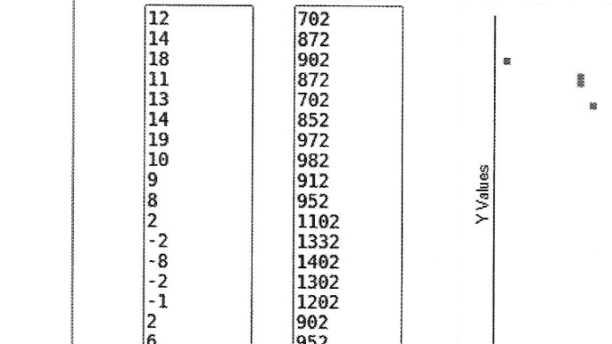
After pasting the data into the online calculator, we received the information that the correlation level amounts to −0.75. This is a high level of interdependence. The lower the temperature outside, the greater the bread sales in the shop. In Analysis 1 it can be seen that a fall in temperature to the level of 2°C, shown in the „X Values” column, causes a rise in bread sales above a thousand loaves.
Analysis 1: Pearson correlation between bread sales and temperature
[A scatter plot from a free online Pearson correlation calculator, plotting X values (temperature, °C) against Y values (loaves sold), with a strongly negative trend — as temperature falls, sales rise; the calculated correlation coefficient is r = −0.75.]
Comparing discrete data
Discrete data is data which cannot be written using fractions, or where there are few unique values. Discrete data includes, for example, the days of the week. If we number the days of the week, we will have 7 unique values, where Monday is one, Tuesday is two, etc. Using discrete values, one cannot calculate a correlation with continuous values. That is, it is incorrect to calculate a correlation between the day of the week and the sales volume.
Temperature is a continuous value; if we wanted to make it into a discrete value, we would have to divide it into temperature ranges, e.g. positive temperature (denoted as 1) and negative (denoted as 0). Discrete format is possessed by the numbers of the days of the month, forming a set of numbers ranging from 1 to 31, a day off and a working day, the season, sun and no sun. It can be assumed that there are more discrete variables than continuous ones.
A red machine brings bad luck. Colour, too, is discrete information; so is bad luck, because we can assume that an accident occurs there once a quarter, or does not.
Since correlation cannot be used to measure the dependency of discrete variables, how does one examine the mutual connections of the data? The t-test comes to our aid.
The t-test
In our case we should make use of the unpaired t-test. The test determines whether there is a difference between two theoretically unconnected groups. The method compares the mean value from two samples. If the difference of the means is large enough, it is assumed that the two groups differ from one another. We can therefore check whether there is a difference in bread sales at temperatures below and above 2°C.
We therefore divide our set from „Analysis 1” into two sets describing the quantity of bread sold. The first describes sales above a temperature above 2°C, the second below.
We enter the data into the online t-test calculator, in the „Treatment 1 (X)” position, bread sales at a temperature above 2°C. We copy into the „Treatment 2 (X)” position the quantity of loaves sold at a temperature below 2°C.
Analysis 2. The t-test between bread sales and temperature
[The online calculator’s output table lists, for Treatment 1 (temperature above 2°C), twelve sales figures around a mean M = 873.25 (SS = 189406.25), and for Treatment 2 (temperature below 2°C), six sales figures around a mean M = 1123.67 (SS = 88083.33).]
The calculator computed a significant difference in the means of both sets, which means that the 2°C temperature boundary has a significant influence on consumer behaviour.
The calculator displayed the following message:
The t-value is -3.80303. The p-value is .000781. The result is significant at p < .05.
The most important information in this message says that the p-value amounts to 0.000781 — that is, it is lower than the threshold of 0.05. This means that the samples differ significantly.
The chi-square test
This is the best-known test for checking the dependency of discrete pairs. In other words, it answers the question: do, for example, older people buy bread more often, do children and adults visit the shop with a different frequency?
Such an analysis may be useful to us, because we can organise free coffee for seniors on Wednesdays, or some other action which will help deepen relations with a defined group of residents. In order to invest resources and all our energy (of which there is always too little), we have to be certain that our assumptions are not „the beliefs of primitive peoples”.
Let us assume that we have divided the residents into 3 age groups: „children and young people”, „adults”, „people 60+”. The shop assistants discreetly record information about the buyer’s age in the sales portal. At the end of the month we have a collected database of the buyers’ age structure.
Table 1: The number of buyers according to age category and day of the week
| Mon | Tue | Wed | Thu | Fri | Sat | |
|---|---|---|---|---|---|---|
| Children and young people | 334 | 334 | 231 | 233 | 543 | 432 |
| Adults | 456 | 345 | 312 | 345 | 343 | 324 |
| Older people | 454 | 347 | 421 | 345 | 532 | 213 |
The data collected during the study can be entered into an online calculator.
Analysis 3. The chi-square test for age categories and days of the week
Degree of freedom (df) = 10
Chi square test (χ²) = 224.008
P value = 0
Since the „P value” amounts to zero (according to my calculations it amounts to 1.5473873958548322e-42), we accept that there are statistically significant differences in shop visits between the three age categories on the individual days of the week.
This means that it is worth investigating the phenomenon further.
Statistical tests are done in order to find out whether the observed phenomenon is significant, or whether it is only our delusion — a so-called „urban legend”. Tests are applied in order to select variables, such as the day of the week, the level of precipitation, or the season, for a regression model. Such a model is easy to work out in free online calculators. It can, with high probability, predict future sales, raw material prices, or the future level of effectiveness of an advertising campaign.
Wojciech Moszczyński
Wojciech Moszczyński — an expert in the field of mathematical optimisation and predictive modelling. For years engaged in popularising econometric methods in business environments. He specialises in optimising sales, production and logistics processes. For 15 years he worked as a financial expert specialising in the area of controlling and management accounting. For 10 years he has worked as a data analyst (data scientist). A graduate of the Department of Econometrics and Statistics of Nicolaus Copernicus University in Toruń. Currently employed as Senior Data Scientist at the Polish company Unity Group.
Dodaj komentarz