Data Science in a Bakery—Grouping Customers of a General Store Using Agglomerative Clustering

Hard times ahead are forcing entrepreneurs to “look at every penny from all sides.” Expenditure must be rational and produce the right results. The decline in consumers’ purchasing power will undoubtedly cause turnover to fall. Combined with rising prices of raw materials and energy, this may spell serious trouble for companies. Intuitively, we know that a decline in sales volume can be partly limited by a very good, accurately targeted marketing offer. We all try to gain a competitive advantage in terms of price and technology and by building customer trust. When we finally manage to create an excellent product or service, our offer must somehow be communicated so that customers have a chance to use it.

This is where the problem of a perfectly competitive market arises. The supply of information is enormous. Customers are showered with offers and promotions and tempted with contests and prizes. Entrepreneurs try to reach the largest possible group of customers. Advertising messages accumulate. Faced with an overwhelming quantity of information, offers and promotions, customers become indifferent. They defend themselves against the noise and advertising clamor, discarding unnecessary information and thereby rendering entrepreneurs’ efforts fruitless.

W-MOSZCZYNSKI-2023-7-47

Segmentation by filtering

The basic way to improve advertising effectiveness is market segmentation. It is a simple and very old way of dividing the customer population into groups. Customers can be divided into women and men, and into old, young and middle-aged people. We distinguish consumer groups by income level and education, or create groups based on place of residence or region. This form of segmentation is called filtering. It can have many levels; for example, we can create a single segment of young female consumers living in rural areas. Young women living in rural areas should receive advertisements in a particular color scheme and containing a particular message developed specifically for this selected consumer group. This solution appears very reasonable.

Unfortunately, there are two serious problems.

1. Lack of attributes for filtering

In online sales, the name on an order enables us to identify the customer’s sex, and the delivery address enables us to identify the place of residence. It will, however, be very difficult to determine age, which is very important when formulating marketing content.

One speaks differently to teenagers than to retired people. An attempt can be made to estimate age by analyzing the goods ordered. Unfortunately, there is no certainty that the order was not placed for a third party.

2. Lack of segment homogeneity

The second problem with segmentation based on filtering is the questionable assumption that all young women living in rural areas will be susceptible to a particular marketing message. These women may, after all, have different temperaments, education and interests. When sending marketing information composed especially for a particular audience, we may feel that we are no longer shooting wide of the mark. This feeling may be very misleading, because the market segment created by filtering will be homogeneous only in appearance.

To summarize, as ChatGPT puts it: “Filtering is the process of selecting particular elements or information from a large dataset on the basis of specified criteria. The purpose of filtering is to eliminate unwanted elements or reduce a dataset to a smaller set containing only the elements that meet specified conditions. Filtering is widely used in data analysis, databases, signal processing, image processing, etc.”

Filtering makes it possible to distinguish particular groups in which people may theoretically have similar preferences. When filtering, we may not have the appropriate consumer attributes available. Furthermore, people placed in a group on the basis of fixed attributes such as age or sex may differ substantially from one another. We may therefore assume that segmentation created through filtering can prove to be an ineffective tool.

Customer segmentation using clusters

How does ChatGPT define this technique?

“Clustering is a data-analysis technique that consists in dividing a dataset into groups (clusters). The objective is to place similar objects in the same cluster and different objects in different clusters. Clustering seeks to find the internal structure of data and discover hidden patterns. It is used in many fields, such as data mining, machine learning, image analysis, etc.” In my view, this definition requires a more detailed discussion.

Let us therefore ask ChatGPT how filtering differs from clustering.

“Clustering is a technique for grouping data into clusters in order to find patterns, whereas filtering consists in selecting or eliminating particular elements from a large dataset on the basis of specified criteria.”

Put more simply, filtering consists in sorting according to specified fixed attributes, whereas clustering consists in grouping based on variable, behavioral attributes. Clustering is not based on fixed attributes such as eye color or place of residence, but on behavior, characteristic habits and certain attributes that are theoretically variable but remain constant over a specified interval of time. I am not sure whether my explanation is simpler than the one presented by ChatGPT.

It is very difficult to explain how the clustering mechanism works, so I created a short example using the Python programming-language environment.

Example of data clustering

A grocery store wants to send marketing offers intended for particular audience groups. The store has no customer information apart from customer ID numbers and email addresses. Five customer groups must be distinguished on the basis of their expenditure in individual product categories.

Using the sales register, a database of 440 transactions made by 100 individual customers was created. Table 1 shows a fragment of this database.

Table 1. Register of product sales by transactions made by individual customers.

ID_customer	Bread	Milk	Industrial goods	Frozen foods	Chemicals	Sweets	Beverages
0	12.67	9.66	10.80	0.71	6.68	2.68	11.57
1	7.06	9.81	13.67	5.87	8.23	3.55	12.20
2	6.35	8.81	10.98	8.02	8.79	15.69	17.53
3	13.26	1.20	6.08	21.35	1.27	8.58	3.14
4	22.62	5.41	10.28	13.05	4.44	10.37	11.15
…	…	…	…	…	…	…	…
435	29.70	12.05	22.90	43.78	0.46	4.41	15.01
436	39.23	1.43	1.09	15.08	0.23	4.69	3.98
437	14.53	15.49	43.20	1.46	37.10	3.78	18.27
438	10.29	1.98	3.19	3.46	0.42	4.25	4.32
439	2.78	1.70	3.59	0.22	1.49	0.10	1.84

440 rows × 8 columns

Next, we create a table of the average expenditure made by each of the 100 customers analyzed.

Table 2. Average customer expenditure in product groups.

PAT = data7.pivot_table(index=['ID_customer'],
    values=['Pieczywo', 'Mleko', 'Art_przemysłowe',
            'Mrożonki', 'Chemia', 'Słodycze', 'Napoje'],
    aggfunc='mean').applymap('{:.2f} zł'.format).reset_index()
PAT

ID_customer	Industrial goods	Chemicals	Milk	Frozen foods	Beverages	Bread	Sweets
0	PLN 3.02	PLN 0.45	PLN 0.70	PLN 0.72	PLN 0.93	PLN 0.42	PLN 0.37
1	PLN 2.65	PLN 1.33	PLN 2.47	PLN 1.90	PLN 2.66	PLN 0.41	PLN 0.12
2	PLN 3.31	PLN 1.98	PLN 2.14	PLN 1.70	PLN 2.61	PLN 0.84	PLN 0.87
3	PLN 6.60	PLN 3.34	PLN 2.31	PLN 1.46	PLN 3.08	PLN 0.60	PLN 1.24
4	PLN 5.02	PLN 3.41	PLN 3.74	PLN 1.34	PLN 4.94	PLN 1.22	PLN 1.91
…	…	…	…	…	…	…	…
95	PLN 36.84	PLN 27.58	PLN 13.37	PLN 24.09	PLN 17.08	PLN 30.52	PLN 5.72
96	PLN 9.37	PLN 3.20	PLN 5.23	PLN 18.88	PLN 9.93	PLN 47.78	PLN 8.40
97	PLN 25.17	PLN 14.41	PLN 15.78	PLN 37.74	PLN 19.05	PLN 36.67	PLN 4.63
98	PLN 25.44	PLN 15.76	PLN 15.58	PLN 51.24	PLN 20.21	PLN 45.22	PLN 7.24
99	PLN 19.42	PLN 4.36	PLN 19.47	PLN 99.14	PLN 34.29	PLN 62.81	PLN 26.21

100 rows × 8 columns

The average values must now be standardized. This is done because an algorithm looking for similarities works incorrectly when values differ drastically from one another. All the numbers in Table 2 will now take values in the interval from 0 to 1.

from sklearn.preprocessing import MinMaxScaler
scaler = MinMaxScaler(feature_range=(0, 1))
PAB = PAT
PAB[['Pieczywo', 'Mleko', 'Art_przemysłowe', 'Mrożonki',
     'Chemia', 'Słodycze', 'Napoje']] = scaler.fit_transform(
    PAB[['Pieczywo', 'Mleko', 'Art_przemysłowe', 'Mrożonki',
         'Chemia', 'Słodycze', 'Napoje']])
PAB

ID_customer	Industrial goods	Chemicals	Milk	Frozen foods	Beverages	Bread	Sweets
0	0.028205	0.4520	0.000000	0.000000	0.000000	0.000304	0.009982
1	0.017530	1.3300	0.081029	0.012004	0.051940	0.000000	0.000000
2	0.036540	1.9780	0.066029	0.009997	0.050366	0.006971	0.021609
3	0.130900	3.3375	0.073381	0.007584	0.064381	0.003165	0.043199
4	0.085566	3.4050	0.139021	0.006314	0.120218	0.012980	0.068774
…	…	…	…	…	…	…	…
95	1.000000	27.5800	0.578758	0.237422	0.484246	0.482509	0.214847
96	0.210647	3.2000	0.206831	0.184592	0.269667	0.759338	0.317720
97	0.664516	14.4080	0.688509	0.376112	0.543111	0.581142	0.173257
98	0.671528	15.7550	0.679559	0.513284	0.578007	0.718195	0.273276
99	0.499274	4.3580	0.857006	1.000000	1.000000	1.000000	1.000000

100 rows × 8 columns

We can now proceed to create the clusters. There is always an optimum number of clusters for specified attributes. This number is found using statistical methods. This time, the number of clusters for the group of 100 customers will be set arbitrarily at 5.

from sklearn.cluster import AgglomerativeClustering
F = PAB[['Pieczywo', 'Art_przemysłowe', 'Chemia', 'Mleko',
         'Mrożonki', 'Napoje', 'Słodycze']].values
cluster = AgglomerativeClustering(n_clusters=5,
    affinity='euclidean', linkage='ward')
PAB['cluster'] = cluster.fit_predict(F)

As a result, each customer in Table 2 is assigned to a particular cluster.

Visualization of clustering

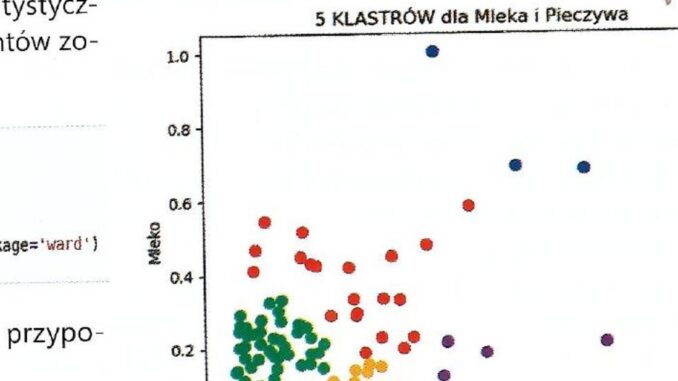
The chart below presents the assignment of customers to clusters for two product groups: milk and bread. Each point on the chart is one of the 100 individual customers. To reflect the quality of the clustering, a seven-dimensional chart would have to be created. This is obviously impossible, so the chart below only imperfectly reflects the five cluster “clouds.” Unfortunately, the algorithm had to “reconcile” as many as seven product types. The chart below presents only two.

plt.figure(figsize=(6, 3))
plt.scatter(PAB['Mleko'], PAB['Pieczywo'], c=cluster.labels_)
plt.ylabel('Mleko')
plt.xlabel('Pieczywo')
plt.title('5 KLASTRÓW dla Mleka i Pieczywa')

To provide more credible evidence of the effectiveness of this method of creating segments, I conducted a clustering analysis exclusively for two products. The previous analysis covered as many as 7 products.

Each point on the chart is an individual customer from the analyzed group of 100 customers. The customers were assigned to one of 5 groups. The groups differ from one another in the average amount spent on bread and milk. The group marked in green spends little money on either milk or bread, while the group marked in purple, consisting of five people, spends substantially more on bread than on milk.

Summary

In today’s era of information noise and declining consumer purchasing power, an effective segmentation method—and, as its consequence, an offer precisely addressed to customers—may prove to be an important competitive advantage. The simple example of clustering-based segmentation presented today demonstrates the great potential of this tool.

Wojciech Moszczyński

Wojciech Moszczyński — an expert in mathematical optimization and predictive modeling. For years, he has been involved in popularizing econometric methods in business environments. He specializes in optimizing sales, production and logistics processes. For 15 years, he worked as a financial expert specializing in controlling and management accounting. For 10 years, he has worked as a data scientist. He is a graduate of the Department of Econometrics and Statistics of Nicolaus Copernicus University in Toruń. He is currently employed as a Senior Data Scientist at the Polish company Unity Group.