

300320201313
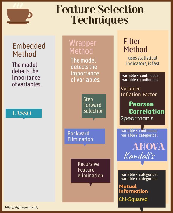
In backward elimination, we start with all the features and removes the least significant feature at each iteration which improves the performance of the model. We repeat this until no improvement is observed on removal of features.
In [1]:
import numpy as np
import pandas as pd
import seaborn as sns
import matplotlib.pyplot as plt
from sklearn.preprocessing import LabelEncoder, OneHotEncoder
import warnings
warnings.filterwarnings("ignore")
from sklearn.model_selection import train_test_split
from sklearn.svm import SVC
from sklearn.metrics import confusion_matrix
np.random.seed(123)
In [2]:
##  colorful prints
def black(text):
     print('33[30m', text, '33[0m', sep='')
def red(text):
     print('33[31m', text, '33[0m', sep='')
def green(text):
     print('33[32m', text, '33[0m', sep='')
def yellow(text):
     print('33[33m', text, '33[0m', sep='')
def blue(text):
     print('33[34m', text, '33[0m', sep='')
def magenta(text):
     print('33[35m', text, '33[0m', sep='')
def cyan(text):
     print('33[36m', text, '33[0m', sep='')
def gray(text):
     print('33[90m', text, '33[0m', sep='')
In [3]:
df = pd.read_csv ('/home/wojciech/Pulpit/6/Breast_Cancer_Wisconsin.csv')
green(df.shape)
df.head(3)
Out[3]:
Deleting unneeded columns
In [4]:
df['concave_points_worst'] = df['concave points_worst']
df['concave_points_se'] = df['concave points_se']
df['concave_points_mean'] = df['concave points_mean']

del df['Unnamed: 32']
del df['diagnosis']
del df['id']
In [5]:
df.isnull().sum()
Out[5]:
In [6]:
import seaborn as sns

sns.heatmap(df.isnull(),yticklabels=False,cbar=False,cmap='viridis')
Out[6]:

Deletes duplicates
there were no duplicates
In [7]:
green(df.shape)
df.drop_duplicates(keep='first', inplace=True)
blue(df.shape)
In [8]:
blue(df.dtypes)
In [9]:
df.columns
Out[9]:
We choose the continuous variable – compactness_mean
In [10]:
print('max:',df['compactness_mean'].max())
print('min:',df['compactness_mean'].min())

sns.distplot(np.array(df['compactness_mean']))
Out[10]:

Backward Elimination
In [18]:
x = df.drop('compactness_mean', axis=1)
y = df['compactness_mean']

from sklearn.model_selection import train_test_split

X_train, X_test, y_train, y_test = train_test_split(X, y, test_size=0.20, random_state=123)
# Jeżeli się rzuca wtedy wycinamy stratify=y.
In [21]:
cols=list(x.columns)
pmax=1
while (len(cols)>0):
    p=[]
    x_1 = x[cols]
    x_1 = sm.add_constant(x_1)
    model=sm.OLS(y,x_1).fit()
    p=pd.Series(model.pvalues.values[1:],index=cols)
    pmax=max(p)
    features_with_p_max=p.idxmax()
    if(pmax>0.05):
        cols.remove(features_with_p_max)
    else:
        break
new_cols=cols
print(new_cols)
In [23]:
df2 = df[new_cols]
blue(df.shape)
df2.head(3)
Out[23]:
The Backward Elimination algorithm stated that reducing variables does not improve the model. Therefore, the number of variables was left unchanged.
OLS linear regression model for variables before reduction
In [12]:
blue(df.shape)
In [13]:
X1 = df.drop('compactness_mean', axis=1)
y1 = df['compactness_mean']
In [14]:
from statsmodels.formula.api import ols
import statsmodels.api as sm

model = sm.OLS(y1, sm.add_constant(X1))
model_fit = model.fit()

print('R2: #blue(model_fit.summary())