

290320202006
Collinearity is the state where two variables are highly correlated and contain similar information about the variance within a given dataset.
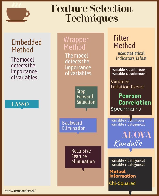
The Variance Inflation Factor (VIF) technique from the Feature Selection Techniques collection is not intended to improve the quality of the model, but to remove the autocorrelation of independent variables.
In [1]:
import numpy as np
import pandas as pd
import seaborn as sns
import matplotlib.pyplot as plt
from sklearn.preprocessing import LabelEncoder, OneHotEncoder
import warnings
warnings.filterwarnings("ignore")
from sklearn.model_selection import train_test_split
from sklearn.svm import SVC
from sklearn.metrics import confusion_matrix
np.random.seed(123)
In [2]:
##  colorful prints
def black(text):
     print('33[30m', text, '33[0m', sep='')
def red(text):
     print('33[31m', text, '33[0m', sep='')
def green(text):
     print('33[32m', text, '33[0m', sep='')
def yellow(text):
     print('33[33m', text, '33[0m', sep='')
def blue(text):
     print('33[34m', text, '33[0m', sep='')
def magenta(text):
     print('33[35m', text, '33[0m', sep='')
def cyan(text):
     print('33[36m', text, '33[0m', sep='')
def gray(text):
     print('33[90m', text, '33[0m', sep='')
In [3]:
df = pd.read_csv ('/home/wojciech/Pulpit/6/Breast_Cancer_Wisconsin.csv')
green(df.shape)
df.head(3)
Out[3]:
Deleting unneeded columns
In [4]:
df['concave_points_worst'] = df['concave points_worst']
df['concave_points_se'] = df['concave points_se']
df['concave_points_mean'] = df['concave points_mean']

del df['Unnamed: 32']
del df['diagnosis']
del df['id']
In [5]:
df.isnull().sum()
Out[5]:
In [6]:
import seaborn as sns

sns.heatmap(df.isnull(),yticklabels=False,cbar=False,cmap='viridis')
Out[6]:

Deletes duplicates
there were no duplicates
In [7]:
green(df.shape)
df.drop_duplicates(keep='first', inplace=True)
blue(df.shape)
In [8]:
blue(df.dtypes)
In [9]:
df.columns
Out[9]:
We choose the continuous variable – compactness_mean
In [10]:
print('max:',df['compactness_mean'].max())
print('min:',df['compactness_mean'].min())

sns.distplot(np.array(df['compactness_mean']))
Out[10]:

Variance Inflation Factor (VIF)
In [11]:
import pandas as pd
import statsmodels.formula.api as smf

def get_vif(exogs, data):
    '''Return VIF (variance inflation factor) DataFrame

    Args:
    exogs (list): list of exogenous/independent variables
    data (DataFrame): the df storing all variables

    Returns:
    VIF and Tolerance DataFrame for each exogenous variable

    Notes:
    Assume we have a list of exogenous variable [X1, X2, X3, X4].
    To calculate the VIF and Tolerance for each variable, we regress
    each of them against other exogenous variables. For instance, the
    regression model for X3 is defined as:
                        X3 ~ X1 + X2 + X4
    And then we extract the R-squared from the model to calculate:
                    VIF = 1 / (1 - R-squared)
                    Tolerance = 1 - R-squared
    The cutoff to detect multicollinearity:
                    VIF > 10 or Tolerance < 0.1
    '''

    # initialize dictionaries
    vif_dict, tolerance_dict = {}, {}

    # create formula for each exogenous variable
    for exog in exogs:
        not_exog = [i for i in exogs if i != exog]
        formula = f"{exog} ~ {' + '.join(not_exog)}"

        # extract r-squared from the fit
        r_squared = smf.ols(formula, data=data).fit().rsquared

        # calculate VIF
        vif = 1/(1 - r_squared)
        vif_dict[exog] = vif

        # calculate tolerance
        tolerance = 1 - r_squared
        tolerance_dict[exog] = tolerance

    # return VIF DataFrame
    df_vif = pd.DataFrame({'VIF': vif_dict, 'Tolerance': tolerance_dict})

    return df_vif
In [12]:
# import warnings
# warnings.simplefilter(action='ignore', category=FutureWarning)
import pandas as pd
from sklearn.linear_model import LinearRegression

def sklearn_vif(exogs, data):

    # initialize dictionaries
    vif_dict, tolerance_dict = {}, {}

    # form input data for each exogenous variable
    for exog in exogs:
        not_exog = [i for i in exogs if i != exog]
        X, y = data[not_exog], data[exog]

        # extract r-squared from the fit
        r_squared = LinearRegression().fit(X, y).score(X, y)

        # calculate VIF
        vif = 1/(1 - r_squared)
        vif_dict[exog] = vif

        # calculate tolerance
        tolerance = 1 - r_squared
        tolerance_dict[exog] = tolerance

    # return VIF DataFrame
    df_vif = pd.DataFrame({'VIF': vif_dict, 'Tolerance': tolerance_dict})

    return df_vif
In [13]:
df.columns
exogs =['radius_mean', 'texture_mean', 'perimeter_mean', 'area_mean',
       'smoothness_mean', 'compactness_mean', 'concavity_mean',
       'concave_points_mean', 'symmetry_mean', 'fractal_dimension_mean',
       'radius_se', 'texture_se', 'perimeter_se', 'area_se', 'smoothness_se',
       'compactness_se', 'concavity_se', 'concave_points_se', 'symmetry_se',
       'fractal_dimension_se', 'radius_worst', 'texture_worst',
       'perimeter_worst', 'area_worst', 'smoothness_worst',
       'compactness_worst', 'concavity_worst', 'concave_points_worst',
       'symmetry_worst', 'fractal_dimension_worst']
In [14]:
print('Jeżeli VIF wynosi więcej niż 5 prawdopodobnie występuje multicollinearity' )

pks = sklearn_vif(exogs, df)
pks.sort_values('VIF').round(1)
print()
blue('LinearRegression in sklearn')
blue(pks[pks['VIF']<=10])


kot = get_vif(exogs, df)
kot.sort_values('VIF').round(1)
print()
green('LinearRegression in statasmodels')
green(kot[kot['VIF']<=10])
OLS linear regression model for variables before reduction
In [15]:
blue(df.shape)
In [16]:
X1 = df.drop('compactness_mean', axis=1)
y1 = df['compactness_mean']
In [17]:
from statsmodels.formula.api import ols
import statsmodels.api as sm

model = sm.OLS(y1, sm.add_constant(X1))
model_fit = model.fit()

print('R2: #blue(model_fit.summary())
OLS linear regression model for variables after reduction
In [22]:
df2 =df[['smoothness_mean','symmetry_mean','texture_se','smoothness_se', 'fractal_dimension_se','symmetry_worst','compactness_mean']]
In [23]:
X2 = df2.drop('compactness_mean', axis=1)
y2 = df2['compactness_mean']
In [24]:
from statsmodels.formula.api import ols
import statsmodels.api as sm

model = sm.OLS(y2, sm.add_constant(X2))
model_fit = model.fit()

print('R2: #blue(model_fit.summary())
red('The reduction of dimensions caused the deterioration of the models properties')