Feature Selection Techniques [categorical result] – Step Forward Selection

010420201017

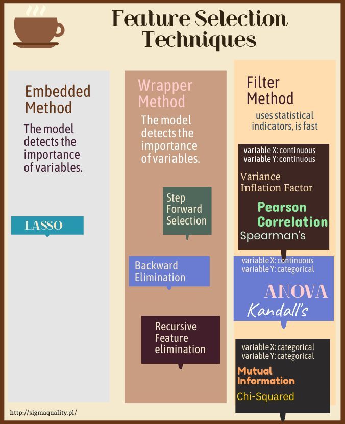
Forward selection is an iterative method in which we start with no function in the model. In each iteration, we add a function that best improves our model until adding a new variable improves the model’s performance.

In [12]:
import numpy as np
import pandas as pd
import seaborn as sns
import matplotlib.pyplot as plt
from sklearn.preprocessing import LabelEncoder, OneHotEncoder
import warnings
warnings.filterwarnings("ignore")
from sklearn.model_selection import train_test_split
from sklearn.svm import SVC
from sklearn.metrics import confusion_matrix
np.random.seed(123)
In [13]:
##  colorful prints
def black(text):
     print('33[30m', text, '33[0m', sep='')  
def red(text):
     print('33[31m', text, '33[0m', sep='')  
def green(text):
     print('33[32m', text, '33[0m', sep='')  
def yellow(text):
     print('33[33m', text, '33[0m', sep='')  
def blue(text):
     print('33[34m', text, '33[0m', sep='') 
def magenta(text):
     print('33[35m', text, '33[0m', sep='')  
def cyan(text):
     print('33[36m', text, '33[0m', sep='')  
def gray(text):
     print('33[90m', text, '33[0m', sep='')
In [14]:
df = pd.read_csv ('/home/wojciech/Pulpit/6/qsar_oral_toxicity.csv', sep=';')
green(df.shape)
df.head(3)
(8991, 1025)
Out[14]:
0 0.1 0.2 0.3 0.4 0.5 0.6 0.7 0.8 0.9 0.962 0.963 0.964 0.965 0.966 0.967 0.968 0.969 0.970 negative
0 0 0 1 0 0 0 0 0 0 0 0 0 0 0 0 0 0 0 0 negative
1 0 0 0 0 0 0 0 0 0 0 0 0 1 0 0 0 0 0 0 negative
2 0 0 0 0 0 0 0 1 0 0 0 0 0 0 0 0 0 0 0 negative

3 rows × 1025 columns

I’m looking for empty cells

In [15]:
import seaborn as sns

sns.heatmap(df.isnull(),yticklabels=False,cbar=False,cmap='viridis')
Out[15]:
<matplotlib.axes._subplots.AxesSubplot at 0x7fca62173d90>
In [16]:
null_value = df.isnull().sum(axis=0)
null_value[null_value != 0]
Out[16]:
Series([], dtype: int64)

Mark empty cells as -999

In [50]:
df.fillna(-999, inplace=True)
In [18]:
df.shape
Out[18]:
(8991, 1025)

Deletes duplicates

there were no duplicates

In [19]:
green(df.shape)
df.drop_duplicates(keep='first', inplace=True)
blue(df.shape)
(8991, 1025)
(8514, 1025)
In [20]:
blue(df.dtypes)
0            int64
0.1          int64
0.2          int64
0.3          int64
0.4          int64
             ...  
0.967        int64
0.968        int64
0.969        int64
0.970        int64
negative    object
Length: 1025, dtype: object
In [21]:
df.columns
Out[21]:
Index(['0', '0.1', '0.2', '0.3', '0.4', '0.5', '0.6', '0.7', '0.8', '0.9',
       ...
       '0.962', '0.963', '0.964', '0.965', '0.966', '0.967', '0.968', '0.969',
       '0.970', 'negative'],
      dtype='object', length=1025)

Encodes the resulting value

In [25]:
df['negative'] = pd.Categorical(df['negative']).codes
df['negative'].value_counts()
Out[25]:
0    7795
1     719
Name: negative, dtype: int64
In [27]:
df.rename(columns={'negative':'ident'}, inplace=True)
df['ident'].head(2)
Out[27]:
0    0
1    0
Name: ident, dtype: int8

Step Forward Selection

In [28]:
X = df.drop('ident', axis=1) 
y = df['ident']  

from sklearn.model_selection import train_test_split

X_train, X_test, y_train, y_test = train_test_split(X, y, test_size=0.20, random_state=123)
# Jeżeli się rzuca wtedy wycinamy stratify=y.
I specify how many programs should indicate the best variables:

In [29]:
k_features = 15
In [30]:
from sklearn.linear_model import LogisticRegression
from mlxtend.feature_selection import SequentialFeatureSelector as sfs

LR = LogisticRegression()

sfs1 = sfs(LR,k_features = k_features, forward=True, floating=False, scoring='r2',verbose=2,cv=5)
sfs1 = sfs1.fit(X_train,y_train)
[Parallel(n_jobs=1)]: Using backend SequentialBackend with 1 concurrent workers.
[Parallel(n_jobs=1)]: Done   1 out of   1 | elapsed:    0.0s remaining:    0.0s
[Parallel(n_jobs=1)]: Done 1024 out of 1024 | elapsed:   39.9s finished

[2020-04-01 09:39:39] Features: 1/15 -- score: -0.09360936522977936[Parallel(n_jobs=1)]: Using backend SequentialBackend with 1 concurrent workers.
[Parallel(n_jobs=1)]: Done   1 out of   1 | elapsed:    0.0s remaining:    0.0s
[Parallel(n_jobs=1)]: Done 1023 out of 1023 | elapsed:   43.9s finished

[2020-04-01 09:40:23] Features: 2/15 -- score: -0.09360936522977936[Parallel(n_jobs=1)]: Using backend SequentialBackend with 1 concurrent workers.
[Parallel(n_jobs=1)]: Done   1 out of   1 | elapsed:    0.0s remaining:    0.0s
[Parallel(n_jobs=1)]: Done 1022 out of 1022 | elapsed:   46.6s finished

[2020-04-01 09:41:09] Features: 3/15 -- score: -0.09360936522977936[Parallel(n_jobs=1)]: Using backend SequentialBackend with 1 concurrent workers.
[Parallel(n_jobs=1)]: Done   1 out of   1 | elapsed:    0.0s remaining:    0.0s
[Parallel(n_jobs=1)]: Done 1021 out of 1021 | elapsed:   50.6s finished

[2020-04-01 09:42:00] Features: 4/15 -- score: -0.0917097195802096[Parallel(n_jobs=1)]: Using backend SequentialBackend with 1 concurrent workers.
[Parallel(n_jobs=1)]: Done   1 out of   1 | elapsed:    0.0s remaining:    0.0s
[Parallel(n_jobs=1)]: Done 1020 out of 1020 | elapsed:   51.1s finished

[2020-04-01 09:42:51] Features: 5/15 -- score: -0.06352720295000061[Parallel(n_jobs=1)]: Using backend SequentialBackend with 1 concurrent workers.
[Parallel(n_jobs=1)]: Done   1 out of   1 | elapsed:    0.1s remaining:    0.0s
[Parallel(n_jobs=1)]: Done 1019 out of 1019 | elapsed:   54.3s finished

[2020-04-01 09:43:45] Features: 6/15 -- score: -0.050378334885553946[Parallel(n_jobs=1)]: Using backend SequentialBackend with 1 concurrent workers.
[Parallel(n_jobs=1)]: Done   1 out of   1 | elapsed:    0.1s remaining:    0.0s
[Parallel(n_jobs=1)]: Done 1018 out of 1018 | elapsed:   58.9s finished

[2020-04-01 09:44:44] Features: 7/15 -- score: -0.035404146912808354[Parallel(n_jobs=1)]: Using backend SequentialBackend with 1 concurrent workers.
[Parallel(n_jobs=1)]: Done   1 out of   1 | elapsed:    0.1s remaining:    0.0s
[Parallel(n_jobs=1)]: Done 1017 out of 1017 | elapsed:  1.0min finished

[2020-04-01 09:45:45] Features: 8/15 -- score: -0.014731021991353432[Parallel(n_jobs=1)]: Using backend SequentialBackend with 1 concurrent workers.
[Parallel(n_jobs=1)]: Done   1 out of   1 | elapsed:    0.1s remaining:    0.0s
[Parallel(n_jobs=1)]: Done 1016 out of 1016 | elapsed:  1.0min finished

[2020-04-01 09:46:46] Features: 9/15 -- score: 0.007752557690146133[Parallel(n_jobs=1)]: Using backend SequentialBackend with 1 concurrent workers.
[Parallel(n_jobs=1)]: Done   1 out of   1 | elapsed:    0.1s remaining:    0.0s
[Parallel(n_jobs=1)]: Done 1015 out of 1015 | elapsed:  1.1min finished

[2020-04-01 09:47:49] Features: 10/15 -- score: 0.034005698374276985[Parallel(n_jobs=1)]: Using backend SequentialBackend with 1 concurrent workers.
[Parallel(n_jobs=1)]: Done   1 out of   1 | elapsed:    0.1s remaining:    0.0s
[Parallel(n_jobs=1)]: Done 1014 out of 1014 | elapsed:  1.1min finished

[2020-04-01 09:48:54] Features: 11/15 -- score: 0.0415299552312852[Parallel(n_jobs=1)]: Using backend SequentialBackend with 1 concurrent workers.
[Parallel(n_jobs=1)]: Done   1 out of   1 | elapsed:    0.1s remaining:    0.0s
[Parallel(n_jobs=1)]: Done 1013 out of 1013 | elapsed:  1.3min finished

[2020-04-01 09:50:10] Features: 12/15 -- score: 0.050864666848338125[Parallel(n_jobs=1)]: Using backend SequentialBackend with 1 concurrent workers.
[Parallel(n_jobs=1)]: Done   1 out of   1 | elapsed:    0.1s remaining:    0.0s
[Parallel(n_jobs=1)]: Done 1012 out of 1012 | elapsed:  1.3min finished

[2020-04-01 09:51:28] Features: 13/15 -- score: 0.058403788853600556[Parallel(n_jobs=1)]: Using backend SequentialBackend with 1 concurrent workers.
[Parallel(n_jobs=1)]: Done   1 out of   1 | elapsed:    0.1s remaining:    0.0s
[Parallel(n_jobs=1)]: Done 1011 out of 1011 | elapsed:  1.3min finished

[2020-04-01 09:52:48] Features: 14/15 -- score: 0.062143619559723404[Parallel(n_jobs=1)]: Using backend SequentialBackend with 1 concurrent workers.
[Parallel(n_jobs=1)]: Done   1 out of   1 | elapsed:    0.1s remaining:    0.0s
[Parallel(n_jobs=1)]: Done 1010 out of 1010 | elapsed:  1.3min finished

[2020-04-01 09:54:09] Features: 15/15 -- score: 0.06776823076716185
In [32]:
feat_cols =list(sfs1.k_feature_idx_)
print(feat_cols)
[0, 1, 2, 67, 93, 231, 426, 506, 512, 526, 558, 559, 696, 795, 939]
In [33]:
PPS = feat_cols

KOT_lasso = dict(zip(df, PPS))
KOT_sorted_keys_lasso = sorted(KOT_lasso, key=KOT_lasso.get, reverse=True)

for r in KOT_sorted_keys_lasso:
    print (r, (KOT_lasso[r]))
0.13 939
0.12 795
0.11 696
0.10 559
1 558
0.9 526
0.8 512
0.7 506
0.6 426
0.5 231
0.4 93
0.3 67
0.2 2
0.1 1
0 0
In [37]:
new_cols = df.columns[feat_cols]
new_cols
Out[37]:
Index(['0', '0.1', '0.2', '0.64', '0.87', '0.218', '0.406', '0.479', '0.485',
       '0.499', '0.530', '0.531', '0.658', '0.751', '0.891'],
      dtype='object')

Creates a dataset with reduced columns

In [39]:
df2 = df[new_cols]
df2['ident']=df['ident']
df2.head(3)
Out[39]:
0 0.1 0.2 0.64 0.87 0.218 0.406 0.479 0.485 0.499 0.530 0.531 0.658 0.751 0.891 ident
0 0 0 1 0 0 0 0 0 0 0 0 0 0 0 0 0
1 0 0 0 0 0 0 0 0 0 0 0 0 0 0 0 0
2 0 0 0 0 0 0 0 0 0 0 0 0 0 0 0 0
In [40]:
# Classification Assessment
def Classification_Assessment(model ,Xtrain, ytrain, Xtest, ytest, y_pred):
    import matplotlib.pyplot as plt
    from sklearn import metrics
    from sklearn.metrics import classification_report, confusion_matrix
    from sklearn.metrics import confusion_matrix, log_loss, auc, roc_curve, roc_auc_score, recall_score, precision_recall_curve
    from sklearn.metrics import make_scorer, precision_score, fbeta_score, f1_score, classification_report

    print("Recall Training data:     ", np.round(recall_score(ytrain, model.predict(Xtrain)), decimals=4))
    print("Precision Training data:  ", np.round(precision_score(ytrain, model.predict(Xtrain)), decimals=4))
    print("----------------------------------------------------------------------")
    print("Recall Test data:         ", np.round(recall_score(ytest, model.predict(Xtest)), decimals=4)) 
    print("Precision Test data:      ", np.round(precision_score(ytest, model.predict(Xtest)), decimals=4))
    print("----------------------------------------------------------------------")
    print("Confusion Matrix Test data")
    print(confusion_matrix(ytest, model.predict(Xtest)))
    print("----------------------------------------------------------------------")
    print(classification_report(ytest, model.predict(Xtest)))
    
    y_pred_proba = model.predict_proba(Xtest)[::,1]
    fpr, tpr, _ = metrics.roc_curve(ytest,  y_pred)
    auc = metrics.roc_auc_score(ytest, y_pred)
    plt.plot(fpr, tpr, label='Logistic Regression (auc = plt.xlabel('False Positive Rate',color='grey', fontsize = 13)
    plt.ylabel('True Positive Rate',color='grey', fontsize = 13)
    plt.title('Receiver operating characteristic')
    plt.legend(loc="lower right")
    plt.legend(loc=4)
    plt.plot([0, 1], [0, 1],'r--')
    plt.show()
    print('auc',auc)

Logistic regression model for variables before reduction

In [41]:
blue(df.shape)
(8514, 1025)
In [42]:
X1 = df.drop('ident', axis=1) 
y1 = df['ident']  


from sklearn.model_selection import train_test_split 

X1_train, X1_test, y1_train, y1_test = train_test_split(X1, y1, test_size=0.20, random_state=123,stratify=y1)
In [43]:
from sklearn.linear_model import LogisticRegression

logmodel = LogisticRegression()
logmodel.fit(X1_train,y1_train)
y1_pred = logmodel.predict(X1_test)
In [44]:
Classification_Assessment(logmodel ,X1_train, y1_train, X1_test, y1_test, y1_pred)
Recall Training data:      0.6887
Precision Training data:   0.9188
----------------------------------------------------------------------
Recall Test data:          0.3958
Precision Test data:       0.6196
----------------------------------------------------------------------
Confusion Matrix Test data
[[1524   35]
 [  87   57]]
----------------------------------------------------------------------
              precision    recall  f1-score   support

           0       0.95      0.98      0.96      1559
           1       0.62      0.40      0.48       144

    accuracy                           0.93      1703
   macro avg       0.78      0.69      0.72      1703
weighted avg       0.92      0.93      0.92      1703

auc 0.6866915223433825

Logistic regression model for variables after reduction

In [45]:
blue(df2.shape)
(8514, 16)
In [47]:
X2 = df2.drop('ident', axis=1) 
y2 = df2['ident']  


from sklearn.model_selection import train_test_split 

X2_train, X2_test, y2_train, y2_test = train_test_split(X2, y2, test_size=0.20, random_state=123,stratify=y2)
In [48]:
from sklearn.linear_model import LogisticRegression

logmodel2 = LogisticRegression()
logmodel2.fit(X2_train,y2_train)
y2_pred = logmodel2.predict(X2_test)
In [49]:
Classification_Assessment(logmodel2 ,X2_train, y2_train, X2_test, y2_test, y2_pred)
Recall Training data:      0.2104
Precision Training data:   0.7707
----------------------------------------------------------------------
Recall Test data:          0.1458
Precision Test data:       0.6562
----------------------------------------------------------------------
Confusion Matrix Test data
[[1548   11]
 [ 123   21]]
----------------------------------------------------------------------
              precision    recall  f1-score   support

           0       0.93      0.99      0.96      1559
           1       0.66      0.15      0.24       144

    accuracy                           0.92      1703
   macro avg       0.79      0.57      0.60      1703
weighted avg       0.90      0.92      0.90      1703

auc 0.569388764165063