

300320202027
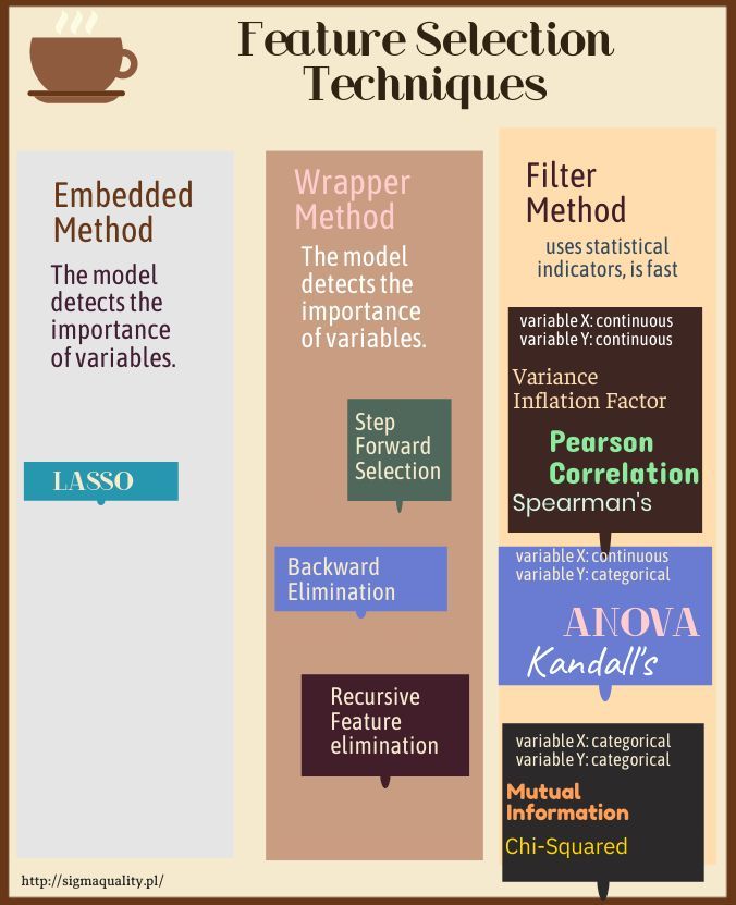
Embedded methods are iterative in a sense that takes care of each iteration of the model training process and carefully extract those features which contribute the most to the training for a particular iteration. Regularization methods are the most commonly used embedded methods which penalize a feature given a coefficient threshold. Here we will do feature selection using Lasso regularization. If the feature is irrelevant, lasso penalizes its coefficient and make it 0. Hence the features with coefficient = 0 are removed and the rest are taken.
import numpy as np
import pandas as pd
import seaborn as sns
import matplotlib.pyplot as plt
from sklearn.preprocessing import LabelEncoder, OneHotEncoder
import warnings
warnings.filterwarnings("ignore")
from sklearn.model_selection import train_test_split
from sklearn.svm import SVC
from sklearn.metrics import confusion_matrix
np.random.seed(123)
##  colorful prints
def black(text):
     print('33[30m', text, '33[0m', sep='')
def red(text):
     print('33[31m', text, '33[0m', sep='')
def green(text):
     print('33[32m', text, '33[0m', sep='')
def yellow(text):
     print('33[33m', text, '33[0m', sep='')
def blue(text):
     print('33[34m', text, '33[0m', sep='')
def magenta(text):
     print('33[35m', text, '33[0m', sep='')
def cyan(text):
     print('33[36m', text, '33[0m', sep='')
def gray(text):
     print('33[90m', text, '33[0m', sep='')
df = pd.read_csv ('/home/wojciech/Pulpit/6/Breast_Cancer_Wisconsin.csv')
green(df.shape)
df.head(3)
Deleting unneeded columns
df['concave_points_worst'] = df['concave points_worst']
df['concave_points_se'] = df['concave points_se']
df['concave_points_mean'] = df['concave points_mean']

del df['Unnamed: 32']
del df['diagnosis']
del df['id']
df.isnull().sum()
import seaborn as sns

sns.heatmap(df.isnull(),yticklabels=False,cbar=False,cmap='viridis')

Deletes duplicates
there were no duplicates
green(df.shape)
df.drop_duplicates(keep='first', inplace=True)
blue(df.shape)
blue(df.dtypes)
df.columns
We choose the continuous variable – compactness_mean
print('max:',df['compactness_mean'].max())
print('min:',df['compactness_mean'].min())

sns.distplot(np.array(df['compactness_mean']))

Lasso
X = df.drop('compactness_mean', axis=1)
y = df['compactness_mean']
I set the number of variables that will remain in the model
Num_v = 15
from sklearn import linear_model

#rlasso = RandomizedLasso(alpha=0.025)

# Standaryzacja zmiennych

clf = linear_model.Lasso(alpha=0.1, positive=True)
clf.fit(X, y)


blue(clf.coef_)
print()
green(clf.intercept_)
print()
red(clf.score(X,y))
The positive parameter, which on Truei forces the coefficients to be positive. In addition, setting alpha regularization to a value close to 0 (i.e., 0.001) causes Lasso to mimic linear regression without regularization.
Metoda zip na wyświetlenie rankingu cech
PPS = clf.coef_

KOT_lasso = dict(zip(df, PPS))
KOT_sorted_keys_lasso = sorted(KOT_lasso, key=KOT_lasso.get, reverse=True)

for r in KOT_sorted_keys_lasso:
    print (r, (KOT_lasso[r]))
We’re adding a result variable
df2 = df[['compactness_mean','texture_worst','perimeter_se']]
df2.head(3)
The Backward Elimination algorithm stated that reducing variables does not improve the model. Therefore, the number of variables was left unchanged.
OLS linear regression model for variables before reduction
blue(df.shape)
X1 = df.drop('compactness_mean', axis=1)
y1 = df['compactness_mean']
from statsmodels.formula.api import ols
import statsmodels.api as sm

model = sm.OLS(y1, sm.add_constant(X1))
model_fit = model.fit()

print('R2: #blue(model_fit.summary())
OLS linear regression model for variables after reduction
blue(df2.shape)
X2 = df2.drop('compactness_mean', axis=1)
y2 = df2['compactness_mean']
from statsmodels.formula.api import ols
import statsmodels.api as sm

model = sm.OLS(y2, sm.add_constant(X2))
model_fit = model.fit()

print('R2: #blue(model_fit.summary())
red('The R2 coefficient is approximately similar to the previously calculated clf.score (X, y).')