

280320200940
Source of data: https://archive.ics.uci.edu/ml/datasets/Air+Quality

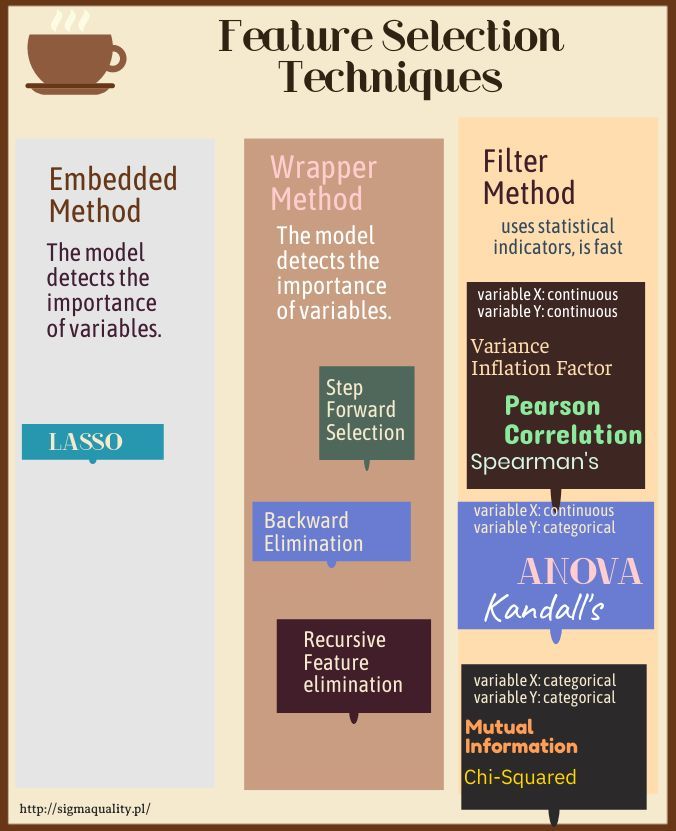
In this case, statistical methods are used:
We always have continuous and discrete variables in the data set.
This procedure applies to the relations of discrete independent variables in relation to discrete result variables.
Below I show the analysis of numerical variables when the resulting value is discrete.
How to Choose a Feature Selection Method For Machine Learning
In [1]:
import numpy as np
import pandas as pd
import seaborn as sns
import matplotlib.pyplot as plt
from sklearn.preprocessing import LabelEncoder, OneHotEncoder
import warnings
warnings.filterwarnings("ignore")
from sklearn.model_selection import train_test_split
from sklearn.svm import SVC
from sklearn.metrics import confusion_matrix
np.random.seed(123)
In [2]:
##  colorful prints
def black(text):
     print('33[30m', text, '33[0m', sep='')
def red(text):
     print('33[31m', text, '33[0m', sep='')
def green(text):
     print('33[32m', text, '33[0m', sep='')
def yellow(text):
     print('33[33m', text, '33[0m', sep='')
def blue(text):
     print('33[34m', text, '33[0m', sep='')
def magenta(text):
     print('33[35m', text, '33[0m', sep='')
def cyan(text):
     print('33[36m', text, '33[0m', sep='')
def gray(text):
     print('33[90m', text, '33[0m', sep='')
In [3]:
df = pd.read_csv ('/home/wojciech/Pulpit/1/AirQualityUCI.csv', sep=';',nrows=1000)
green(df.shape)
df.head(3)
Out[3]:
Usuwanie niepotrzebnych kolumn
In [4]:
del df['Unnamed: 15']
del df['Unnamed: 16']
Kasuje brakujące rekordy
In [5]:
green(df.shape)
df.isnull().sum()
df = df.dropna(how='any')
blue(df.shape)
blue(df.isnull().sum())
Kasuje duplikaty
nie było duplikatów
In [6]:
green(df.shape)
df.drop_duplicates(keep='first', inplace=True)
blue(df.shape)
Z daty wyciągam dzień tygodnia, miesiąc, oraz godzinę jako zmienne ciągłe
In [7]:
df['Date'] = pd.to_datetime(df.Date)
df['day'] = df['Date'].dt.weekday
df['month'] = df['Date'].dt.month
df['hour'] = df['Time'].str.slice(0,2)
df[['Date','day','month','hour']].head(3)
Out[7]:
In [8]:
del df['Date']
del df['Time']
Kasuje zmienną -200 oznaczającą błąd danych
In [9]:
df[['CO(GT)', 'PT08.S1(CO)', 'NMHC(GT)', 'C6H6(GT)', 'PT08.S2(NMHC)',
       'NOx(GT)', 'PT08.S3(NOx)', 'NO2(GT)', 'PT08.S4(NO2)', 'PT08.S5(O3)',
       'T', 'RH', 'AH', 'day', 'month', 'hour']] = df[['CO(GT)', 'PT08.S1(CO)', 'NMHC(GT)', 'C6H6(GT)', 'PT08.S2(NMHC)',
       'NOx(GT)', 'PT08.S3(NOx)', 'NO2(GT)', 'PT08.S4(NO2)', 'PT08.S5(O3)',
       'T', 'RH', 'AH', 'day', 'month', 'hour']].replace(-200,np.NaN)
In [10]:
df.isnull().sum()
Out[10]:
In [11]:
del df['NMHC(GT)']
green(df.shape)
df.isnull().sum()
df = df.dropna(how='any')
blue(df.shape)
blue(df.isnull().sum())
Zamieniam zmienne na wartości numeryczne
In [12]:
blue(df.dtypes)
Macierz korelacji
In [13]:
df['CO(GT)'] = df['CO(GT)'].str.replace(',', '.')
In [14]:
df['C6H6(GT)'] = df['C6H6(GT)'].str.replace(',', '.')
In [15]:
df['T'] = df['T'].str.replace(',', '.')
In [16]:
df['RH'] = df['RH'].str.replace(',', '.')
In [17]:
df['AH'] = df['AH'].str.replace(',', '.')
In [18]:
df[['CO(GT)', 'PT08.S1(CO)', 'C6H6(GT)', 'PT08.S2(NMHC)',
       'NOx(GT)', 'PT08.S3(NOx)', 'NO2(GT)', 'PT08.S4(NO2)', 'PT08.S5(O3)',
       'T', 'RH', 'AH', 'day', 'month', 'hour']] = df[['CO(GT)', 'PT08.S1(CO)', 'C6H6(GT)', 'PT08.S2(NMHC)',
       'NOx(GT)', 'PT08.S3(NOx)', 'NO2(GT)', 'PT08.S4(NO2)', 'PT08.S5(O3)',
       'T', 'RH', 'AH', 'day', 'month', 'hour']].astype(float)
In [19]:
CORREL = df.corr()
plt.figure(figsize=(10,6))
sns.heatmap(CORREL, annot=True, cbar=False, cmap="coolwarm")
Out[19]:

Koduje zmienną kategoryczną wynikową – C6H6(GT)
In [20]:
print('max:',df['C6H6(GT)'].max())
print('min:',df['C6H6(GT)'].min())

sns.distplot(np.array(df['C6H6(GT)']))
Out[20]:

In [21]:
df['C6H6(GT)'] = df['C6H6(GT)'].apply(lambda x: 1 if x > 10 else 0)
df['C6H6(GT)'].value_counts()
Out[21]:
In [22]:
df['C6H6(GT)'] = pd.Categorical(df['C6H6(GT)']).codes
df['C6H6(GT)'].value_counts()
Out[22]:
Model regresji liniowej bez redukcji zmiennych
In [23]:
blue(df.dtypes)
In [24]:
X = df.drop('C6H6(GT)', axis=1)
y = df['C6H6(GT)']
Podział na dane treningowe i testowe
In [25]:
from sklearn.model_selection import train_test_split

X_train, X_test, y_train, y_test = train_test_split(X, y, test_size=0.20, random_state=123,stratify=y)
Definicje
In [26]:
# Classification Assessment
def Classification_Assessment(model ,Xtrain, ytrain, Xtest, ytest, y_pred):
    import matplotlib.pyplot as plt
    from sklearn import metrics
    from sklearn.metrics import classification_report, confusion_matrix
    from sklearn.metrics import confusion_matrix, log_loss, auc, roc_curve, roc_auc_score, recall_score, precision_recall_curve
    from sklearn.metrics import make_scorer, precision_score, fbeta_score, f1_score, classification_report

    print("Recall Training data:     ", np.round(recall_score(ytrain, model.predict(Xtrain)), decimals=4))
    print("Precision Training data:  ", np.round(precision_score(ytrain, model.predict(Xtrain)), decimals=4))
    print("----------------------------------------------------------------------")
    print("Recall Test data:         ", np.round(recall_score(ytest, model.predict(Xtest)), decimals=4))
    print("Precision Test data:      ", np.round(precision_score(ytest, model.predict(Xtest)), decimals=4))
    print("----------------------------------------------------------------------")
    print("Confusion Matrix Test data")
    print(confusion_matrix(ytest, model.predict(Xtest)))
    print("----------------------------------------------------------------------")
    print(classification_report(ytest, model.predict(Xtest)))

    y_pred_proba = model.predict_proba(Xtest)[::,1]
    fpr, tpr, _ = metrics.roc_curve(ytest,  y_pred)
    auc = metrics.roc_auc_score(ytest, y_pred)
    plt.plot(fpr, tpr, label='Logistic Regression (auc = plt.xlabel('False Positive Rate',color='grey', fontsize = 13)
    plt.ylabel('True Positive Rate',color='grey', fontsize = 13)
    plt.title('Receiver operating characteristic')
    plt.legend(loc="lower right")
    plt.legend(loc=4)
    plt.plot([0, 1], [0, 1],'r--')
    plt.show()
    print('auc',auc)
In [27]:
blue(X.shape)
green(X_train.shape)
green(X_test.shape)
Modelu klasyfikacji bez wyboru funkcji
In [28]:
import numpy as np
from sklearn import model_selection
from sklearn.pipeline import make_pipeline
from sklearn.linear_model import LogisticRegression
from sklearn.model_selection import GridSearchCV

Parameteres = {'C': np.power(10.0, np.arange(-3, 3))}
LR = LogisticRegression(warm_start = True)
LR_Grid = GridSearchCV(LR, param_grid = Parameteres, scoring = 'roc_auc', n_jobs = -1, cv=2)

LR_Grid.fit(X_train, y_train)
y_pred_LRC = LR_Grid.predict(X_test)
In [29]:
Classification_Assessment(LR_Grid ,X_train, y_train, X_test, y_test, y_pred_LRC)

Redukcja zmiennych niezależnych za pomocą OLS
In [30]:
from statsmodels.formula.api import ols
import statsmodels.api as sm

model = sm.OLS(y, sm.add_constant(X))
model_fit = model.fit()

blue(model_fit.summary())
In [31]:
p_values = model_fit.summary2().tables[1]['P>|t|']
## zaokrąglam


p_values = np.round(p_values, decimals=2)
p_values= p_values.sort_values()

plt.figure(figsize=(3,8))
p_values.plot(kind='barh')
plt.title('p-value for independent variables in OLS')
plt.grid(True)
plt.ylabel('independent variables')
plt.xlabel('p-value')
plt.xticks(rotation=90)
Out[31]:

Wybieramy zmienne z p-value < 0.1
In [32]:
df.columns
Out[32]:
In [33]:
df2= df[['PT08.S4(NO2)','PT08.S3(NOx)','PT08.S2(NMHC)','AH','C6H6(GT)']]
In [34]:
y= y.to_frame()
y.head(4)
Out[34]:
In [35]:
fig = plt.figure(figsize = (20, 25))
j = 0
for i in df2.columns:
    plt.subplot(6, 4, j+1)
    j = 1+j
    sns.distplot(df2[i][y['C6H6(GT)']==0], color='#999999', label = '0')
    sns.distplot(df2[i][y['C6H6(GT)']==1], color='#ff0000', label = '1')
    plt.legend(loc='best',fontsize=10)
fig.suptitle('Classification charts',fontsize=34,color='#ff0000',alpha=0.3)
fig.tight_layout()
fig.subplots_adjust(top=0.95)
plt.show()

In [36]:
def scientist_plot(data, y, AAA, Title):
    fig = plt.figure(figsize = (20, 25))
    j = 0
    for i in df2.columns:
        plt.subplot(6, 4, j+1)
        j = 1+j
        sns.distplot(data[i][y[AAA]==0], color='#999999', label = '0')
        sns.distplot(data[i][y[AAA]==1], color='#274e13', label = '1')
        plt.legend(loc='best',fontsize=10)
    fig.suptitle(Title,fontsize=34,color='#274e13',alpha=0.5)
    fig.tight_layout()
    fig.subplots_adjust(top=0.95)
    plt.show()
In [37]:
scientist_plot(df2, y, 'C6H6(GT)','Classification charts')

In [38]:
fig = plt.figure(figsize = (20, 25))
kot = ['#999999','#274e13']
sns.pairplot(data=df2[['PT08.S4(NO2)','PT08.S3(NOx)','PT08.S2(NMHC)','AH','C6H6(GT)']], hue='C6H6(GT)', dropna=True, height=2, palette=kot)
fig.suptitle('Classification charts',fontsize=34,color='#274e13',alpha=0.3)
fig.tight_layout()
fig.subplots_adjust(top=0.95)
plt.show()
